Resources for students in Stat 111 (Spring 2023). Managed by aL Xin.
View files on GitHub awqx/stat111-2023
SectionsLectures
Exam materials
R Bootcamp
Syllabus
I use Windows, so I may get some MacOS shortcuts wrong.
To get the most mileage from this document, I suggest having both the R Markdown file open alongside the PDF or webpage. By default, the chunks are set to not evaluate using eval = F (see the source). If you want to see results from each chunk, remove eval = F from the very first chunk in the source .Rmd file and recompile the document.
If you have additional questions, email me at axin@college.harvard.edu.
Looking for the practice problems? Click here.
What is R Markdown?
R Markdown is a file format that integrates text editing and R code evaluation. Using R Markdown, you can create reports with formatted text, LaTeX and R.
R Markdown files have the extension .Rmd. You can view the contents within any text editor (not necessarily RStudio). However, RStudio provides convenient integration of R with the files.
R code in .Rmd lives in chunks, which are sandwiched by three grave accents. You can create a chunk by going to the menu bar and selecting Code > Insert Chunk, using the drop down next to Insert at the top right of the file and selecting R, or using the shortcut Ctrl + Alt + I in Windows or Ctrl + Option + I in MacOS.
To run the code in a single chunk, press the green play button in the upper right of the chunk. You can also use Ctrl + Shift + Enter (Windows) or Cmd + Shift + Return (MacOS). To run a single line, select the line and use Ctrl + Enter or Cmd + Return.
In RStudio, you can “knit” R Markdown files to produce documents that execute the code within all the chunks, and incorporates it into a single document along with the text and LaTeX. You can knit the file using the button in the top right or using the keyboard shortcut Ctrl + Shift + K or Cmd + Shift + K in MacOS.
LaTEX
To use LaTEX in R Markdown, you need to install a compatible LaTEX engine. I think tinytex is the best option here because it’s hasslefree. Here’s how you’d load it into R:
install.packages("tinytex")
tinytex::install_tinytex()
1 R Basics
Some features of R:
- R is case-sensitive
- Indexing begins with 1
- Comments start with pound signs
#
1.1 Arithmetic
Arithmetic in R automatically follows order of operations. Symbols are consistent with most other coding languages.
# Demonstration of arithmetic
# This equals 111
11 + 4 * 5 ^ 2
# Modulo (remainder) in R
139560 %% 2021
1.2 Data types
The most important data types we’ll use are:
- Logical:
TRUE,FALSE,T,F - Integer:
110,111 - Numeric:
6.036 - Character:
"Conditioning is the soul of statistics"
R does type assignment automatically; just assign whatever value you need to a variable name. Assignment is accomplished using an arrow, i.e., <-. Standard practice is to use left arrows (as demonstrated), though right arrows also work. It is possible to assign using =, but it is discouraged.
You can check data type with the function class().
# Create a numeric variable approximately equal to sqrt(2)
x <- 1.41421
x = 1.41421 # discouraged, but possible
# This is equivalent to 1.41421 -> x
class(x)
1.3 Vectors
R’s most useful data structures are vectors. These are finite ordered sequences of elements of a single data type (similar to tuples in Python).
Create vectors using the function c(). Index a vector to obtain its components using square brackets. Recall that indexing in R begins with 1, not 0. You can also modify the vector’s components using indexing.
Remove elements of a vector through indexing with negative integers.
x <- c("hydrogen", 1, 1.01, "gas")
x[1]

# Notice that 1, 1.001, and x are coerced to "character"
class(x)
class(x[2])

# Modify components
x[3] <- 1.008
x

# Delete components
x <- x[-4]
x

# Insert components
x <- c(x, "helium")

# Insert components in the middle
x <- c(x[1:2], "third", x[3:5])
x
You can also name the components of a vector and index based on name, though this is also rarely used in STAT 111.
names(x) <- c("name", "number", "mass")
x["number"]
1.3.1 Vector arithmetic
Vectors in R support element-wise operations, which is best illustrated through examples.
# Arithmetic of vectors of the same length
c(50, 51, 61) + c(110, 111, 139)

# Arithmetic with vectors of differing lengths
# Shortest vector is recycled (warning if not whole multiple)
c(121, 124) + c(110, 111, 139)
c(121, 124) + c(104, 110, 111, 139)

# Arithmetic with constants
2 * c(110, 111, 139)
c(1, 2, 3) * c(110, 111, 139)
100 + c(10, 11, 39)
1.4 Equality
Standard practice in R is to use <- when assigning a value to a variable. When checking for equality, use ==, i.e., x == 2. When assigning arguments, use single equals signs. For example, mean(c(1, 2, 3, NA), na.rm = T).
c(110, 51, 61) == c(110, 111, 139)
1.5 Lists
For more flexibility, we can use lists, which are ordered collections of elements that can contain more than one data type (including other lists).
Create lists using list(). The components of lists can also be named. Index lists with double square brackets.
# Instead of using names(), you can create lists with components already named
# The same applies for vectors
x <- list(
  name = "hydrogen",
  number = 1,
  mass = 1.008
)

x[[1]]
x[["number"]]
# Here, 1 is not coerced to a character
class(x[["number"]])
1.6 Exercise 1: Variance of a vector
Create a vector temp and return its sample variance.
Sample variance can be calculated for a vector using the function var(). Check the results of your calculation against var(temp).
Recall that sample variance is calculated as
\[ \text{Var}(\mathbf{x}) = \frac{1}{n-1}\sum_{i = 1}^n (x_i - \bar{x})^2. \]
If you look at the .Rmd source here, you’ll see a good example of how to format LaTeX in the file. For display style equations, use double dollar signs; for inline style equations, use single dollar signs.
set.seed(111)
x <- rnorm(11234)
1/(length(x) - 1) * sum((x - mean(x))^2)
var(x)
cat(
  "Our function:", 1/(length(x) - 1) * sum((x - mean(x))^2), "\n",
  "Built-in var():", var(x)
)
1.7 Packages
To install R packages, use the function install.packages() with the package name in quotes. After a package has been installed, you can use its functions using double colon notation. For example, if we wanted to use str_detect() from stringr to find patterns of characters, we could write stringr::str_detect(). This can become a hassle, so you can load all the functions in a package with library(stringr).
2. Probability distributions in R
R has built-in functions for working with many probability distributions covered in STAT 111. For any family of distributions in R (Binomial, Normal, etc.), there are four functions. For example, with Normal distributions, we have:
dnorm(x, mean = mu, sd = sigma): Returns the probability density evaluated atxfor a Normal distribution with meanmuand standard deviationsigma. Be careful to specify the standard deviation, not the variance.- This is equivalent to $ \phi((x - \mu)/\sigma) $
pnorm(q, mean = mu, sd = sigma): Returns the CDF evaluated atq.- Equivalent to $\Phi((x - \mu)/\sigma) $
qnorm(p, mu, sigma): Returns the value corresponding to $p $th quantile.rnorm(n, my, sigma): Returns $n $ i.i.d. observations from the Normal r.v.
The prefixes d, p, q, and r and the first arguments are consistent between probability distributions. However, different distributions require additional arguments to be specified. For example, to generate 10 i.i.d. observations with distribution \text{Bin}(n, p), we would use the function call rbinom(10, size = n, prob = p).
# What are the outputs for each of these?
dnorm(0)
pnorm(0)
qnorm(0)
rnorm(10)
2.1 Exercise 2: Law of large numbers
Recall that the Law of Large Numbers (LLN) states that the sample mean of i.i.d. observations approaches the expected value as the sample size increases.
Choose a distribution and generate samples of various sizes to observe the LLN.
x <- lapply(
  c(10 * c(1:10), 1000, 10000, 100000),
  rexp,
  rate = 1
)

y <- lapply(x, mean)
3. Tabular data
3.1 Matrices
Matrices in R can be created using matrix(). The first argument is a vector containing the data for the matrix. The second argument is the number of rows or columns and whether the data should be read by row or by column. Default behavior is to read data by columns.
X <- matrix(c(1, 1, 0, 1, 1, 1, 1, 3, 9), nrow = 3, byrow = T)
X
R can handle various matrix operations. First, indexing can be accomplished using single square brackets. First element is row, and second element is column.
# Get a row of the matrix
X[1, ]

# Get a column of the matrix
X[, 1]

# Get the dimensions of X (row, col)
dim(X)

# Create the transpose of X
Xt <- t(X)

# Matrix multiplication
XtX <- Xt %*% X

# Find the inverse of a matrix
XtX_inverse <- solve(XtX)

# Sanity check (notice zero can sometimes be a very small number)
XtX %*% XtX_inverse
Matrices can be modified like vectors, though indexing for a single element requires both the row and column coordinate.
# Change a single element at the [2,2] position
X[2, 2] <- 5

# Replace the first row
X[1, ] <- c(2, 2, 3)

# Remove the last column
X <- X[, -3]

# Reset the matrix
X <- matrix(c(1, 1, 0, 1, 1, 1, 1, 3, 9), nrow = 3, byrow = T)
3.2 Data frames
Data frames are more flexible than matrices. They can be created from matrices or created by supplying the columns. The two methods shown below create the same data frame.
Y <- data.frame(X)
names(Y) <- c("Q", "W", "E")
Y
X

Y <- data.frame(
  Q = c(1, 1, 1),
  W = c(1, 1, 3),
  E = c(0, 1, 9)
)
Y
Structurally, data frames are lists of vectors, where each vector corresponds to a column. So, while a data frame can contain many data types, each column corresponds to only one data type. We can access the columns of a data frame by name using the dollar sign, double brackets, or single brackets. Rows can also be retrieved and modified with similar operations.
By supplying elements to a new index, you can also add elements to the data frame.
# The following commands return the same element: the first column of Y
Y[["Q"]]
Y[[1]]
Y$Q
Y[, "Q"]

# Rows can also be named and indexed that way
# Rows cannot use dollar sign notation or double brackets
# The following all return the first row of Y
rownames(Y) <- c("A", "S", "D")
Y["A", ]
Y[1, ]

# The following both return the middle element of Y
Y[2, 2]
Y["S", "W"]

# Either of the following would add the the column `R`
# This is added to the end of the data frame
Y[, 4] <- c("Joe", "Joe and Neil", "Kevin")
names(Y)[4] <- "R"

Y$R <- c("Joe", "Joe and Neil", "Kevin")

# Remove the column
Y <- Y[, -4]
We can filter data frames by supplying Boolean vectors when indexing. Additionally, because of the helpful element-wise properties of R vectors, we can use this property to sort data frames.
# We want rows of the data frame where the second element is 1
Y[Y$W == 1, ]
3.3 Exercise 3: Datasets in R
R has a variety of example data sets that you can look through using the function data(). Take a look at the data set iris, which you can view by entering iris. (Think of the data set as an “invisible” variable that contains the data frame.)
Which of the flower species has the widest petals, on average?
See answer
Virginica. There are a few ways to solve this, one of which involves taking the average of every single group. For example,
mean(iris[iris$Species == "virginica", "Petal.Length"]). There's a "cleaner" solution in Section 3.5.
3.4 Miscellaneous useful commands
To view the first few rows of a data frame or first few elements of a vector/list, use head(). To view the last elements, use tail(). You can supply an optional second argument specifying the number of elements you want to see.
head(iris, 3)
3.5 Further reading
There are more advanced (and convenient, if you want to put time into learning) ways of sorting data frames using the packages tibble, dplyr, and tidyr. These will largely not be necessary for STAT 111, though reach out if you want any tips!
For example, we can use dplyr to solve Exercise 3 with:
library(dplyr)
iris %>%
  group_by(Species) %>%
  summarize(petal_width_avg = mean(Petal.Width), .groups = "drop") %>%
  top_n(1, petal_width_avg) %>%
  .$Species
4 Iteration
4.1 For loops
For loops are common in STAT 111. They allow you to run some code for every element in a collection. For example:
my_vector <- c(110, 111, 139) # Numbers 1 through 10
for (i in my_vector) {
  print(i %% 17)
}
4.2 Vectorized operations
For loops can be useful but are usually not the most efficient solution. For example, we could accomplish the same task as the example in 4.1 with a single vector operation.
my_vector %% 17
4.3 Replicate
The function replicate repeatedly evaluates an expression. This is useful for simulations. For example, if our experiment was to observe 10 i.i.d. r.v.s with an Exponential distribution with $\lambda = 1 $, we can replicate the experiment 100 times using the following:
# run the code to see how simplify changes the result
result <- replicate(100, rexp(10, 1), simplify = F)
result <- replicate(100, rexp(10, 1), simplify = T)
4.4 Exercise 4: Central Limit Theorem (CLT)
Observe the CLT in action with simulations!
Generate 500 trials of observing 5 i.i.d. Exponential r.v.s with $\lambda = 1 $. Find the mean of each trial and plot the histogram of the sample means using hist(vector.name).
Repeat the above with 50 and 1000 r.v.s (not replications).
Hint: Define a separate vector to store the means.
trial <- function() {
 x <- rexp(50, 1)
 mean(x)
}
result <- replicate(500, trial())
hist(result)
5 Functions and control flow
5.1 Creating functions
Replication is most useful when combined with custom functions. We can define a function to find the element with the highest magnitude in a vector like so:
# We can set default values to arguments in functions, like na.rm here
max_magnitude <- function(vec, na.rm = T) {
  max(abs(vec), na.rm = na.rm)
}
max_magnitude(c(NA, -50, 51, -61, 121, -124))
5.2 Control flow
R uses fairly intuitive control flow with notation for if, else if, and else. Additionally, a value of 0 evaluates to FALSE and any other value evaluates to TRUE.
for (i in 1:5) {
  if (i %% 2) {
    message(i, " is odd")
  } else {
    message(i, " is even")
  }
}
R also has switch-case capabilities, though it is unlikely to be used in this class.
5.3 Exercise 5: CLT Revisited
Instead of a for loop, can you get the vector of means using a single call to replicate?
6 Plotting
R has base functions for plotting, but I personally dislike them. Instead, we’ll be using ggplot2.
6.1 Creating a scatterplot
# install ggplot2 if you haven't already
# install.packages(ggplot2)
library(ggplot2)

# Let's generate some example data
predictor <- rnorm(10)
response <- 10 + 2*predictor + rnorm(10, 0, .5)
# Create a data frame of data
df <- data.frame(predictor, response)

ggplot(data = df, aes(x = predictor, y = response)) +
  geom_point() + # create points with x and y
  # create blue linear regression line
  geom_smooth(method = "lm", se = F, color = "blue") +
  # create red true regression line
  geom_abline(slope = 2, intercept = 10, color = "red") +
  # make it pretty (optional)
  theme_bw()
6.2 Creating a histogram
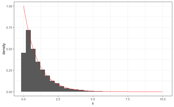
We can generate 400 samples from an Exponential distribution with $\lambda = 1 $ and see how the histogram compared to the known PDF of the distribution.
# Generate samples of data
expo_samp <- rexp(10000, 1)
expo_samp_df <- data.frame(expo_samp)

# Generate known PDF
x <- seq(0, 7, by = 0.01)
expo_pdf <- dexp(x, 1)
expo_df <- data.frame(x, expo_pdf)

ggplot(data = expo_samp_df, aes(x = expo_samp)) +
  # An ordinary histogram would not have the additional aes() arg
  geom_histogram(aes(y = ..density..)) +
  # Add a line for the PDF (use different data)
  geom_line(data = expo_df, aes(x = x, y = expo_pdf), color = "red") +
  theme_bw()
6. Equivalent functions in base R
If you’re curious about how to do the same things using base R (without needing to install ggplot2) here’s a brief summary.
# Make a scatter plot with the same data
plot(
 predictor,
 response,
 xlab = "Predictor",
 ylab = "Response"
) +
# Add calculated linear regression line
abline(lm(response ~ predictor), col = "blue") +
# Add true regression line
abline(10, 2, col = "red")

# Make a histogram with the same data
# To make a normal histogram, set freq = T
hist(expo_samp, freq = F) +
curve(dexp(x, 1), col = "red", add = T)
Practice problems
1 Maximum likelihood estimator
We’re often concerned with finding the value of a parameter that maximizes the probability of observing the data that we did. This is called a maximum likelihood estimate or MLE. Let’s use an example to visualize maximum likelihood.
1.1 Generate data
Create 20 random observations from a Poisson r.v. with rate parameter 3. Suppose we know that the data are i.i.d. Poisson observations but we don’t know the rate parameter. (Consider: is this a realistic scenario?)
For each rate parameter from 0.01 to 5.00 (in 0.01 increments), find the likelihood of your data.
Save these likelihoods in some vector.
Solution:
set.seed(111)
x <- rpois(10000, 3)
lambdavec <- seq(0.01, 5, 0.01)

get_poislik <- function(xvec, lambda) sum(dpois(xvec, lambda))

poislik <- sapply(
	lambdavec,
	get_poislik,
	xvec = x
)
1.2 Plot likelihood
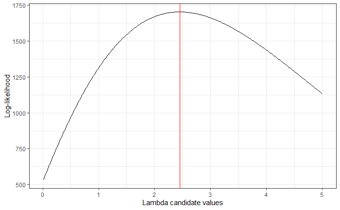
Now, make a line plot of the rate parameters versus the likelihoods. What appears to be the value of $ \lambda $ that maximizes the likelihood? Plot a vertical line at that rate parameter.
Solution: Note that we use which.max in order to grab the correct index of the maximum and then grab the correct value of our rate parameter.
# install.packages("ggplot2") # if you haven't already
library(ggplot2)
q12 <- data.frame(lambda = lambdavec, lik = poislik)

ggplot(q12, aes(x = lambda, y = lik)) +
	geom_line() +
	geom_vline(xintercept = lambdavec[which.max(poislik)], color = "red") +
	theme_bw() +
	labs(
		x = "Lambda candidate values",
		y = "Log-likelihood"
	)
2 Biased sample variance
The sample variance of i.i.d. observations $ X_1, \dots, X_n $ with true variance $ \sigma^2 $ is given by
\[ \hat{\sigma}^2 = \frac{1}{n-1}\sum_{i = 1}^n (x_i - \bar{x})^2. \]
The estimator $ \hat{\sigma}^2 $ is unbiased in that its expectation is the true variance, i.e. $ E(\hat{\sigma}^2) = \sigma^2 $. This problem shows that $ \hat{\sigma}^2 $ is unbiased while the estimator determined by $ \frac{1}{n}\sum_{i = 1}^n(X_i - \bar{X})^2 $ is.
2.1
Create a function that calculates $ \hat{\sigma}^2_n $ for any vector of data.
Solution: Checking the documentation, we see that we can adapt the base R function var for our purposes.
var_new <- function(x) var(x) * (length(x) - 1) / length(x)
2.2
Using 10 000 iterations, run a for loop that generates $ n = 10 $ independent observations from a Standard Normal r.v. and calculates $ \hat{\sigma}^2_{n-1} $ and $ \hat{\sigma}^2_n $. On average, which estimator is closer to the true value, $ \sigma^2 = 1 $.
Solution: We can print a result that will be knitted in the PDF using the cat function to concatenate text and output.
Note that we’re taking the matrix result of replicate and converting it to a data.frame to use sapply.
q22 <- data.frame(replicate(10000, rnorm(10)))
sigma_n1 <- sapply(q22, var)
sigma_n <- sapply(q22, var_new)

cat(
	"n:", mean(sigma_n - 1), "\n",
	"n - 1:", mean(sigma_n1 - 1)
)
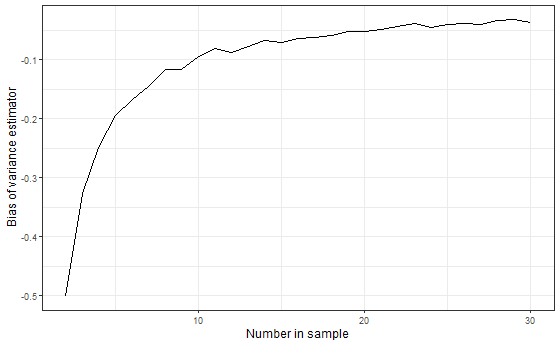
2.3 (Challenge)
Let’s see how the bias of $ \hat{\sigma}^2_n $ varies with the sample size $ n $. Using $ n = 2, 3, …, 30 $, do the following 100 times: generate $ n $ independent observations from a Standard Normal and calculate $ \hat{\sigma}^2_n $. Then plot $ n $ vs. the average $ \hat{\sigma}^2_n - \sigma^2 $ for each value $ n $. (Note: we have two loops here: one for each size $ n $ and one inner-loop that calculates 100 samples of size $ n $ for each $ n $).
Solution:
library(dplyr) # gives us the pipe "%>%"
nsamp <- c(2:30)
get_n <- function(nsamp) {
	temp <- replicate(10000, rnorm(nsamp)) %>%
		data.frame() %>%
		sapply(var_new)
	mean(temp - 1)
}
q2_3 <- data.frame(nsamp, bias = sapply(nsamp, get_n))
ggplot(q2_3, aes(x = nsamp, y = bias)) +
	geom_line() +
	labs(
		x = "Number in sample",
		y = "Bias of variance estimator"
	)
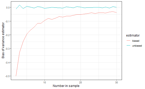
As a bonus, we can also do the same calculations for the unbiased estimator and compare them. This code shows one of several ways you could combine the two lines on one graph.
get_n1 <- function(nsamp) {
	temp <- replicate(10000, rnorm(nsamp)) %>%
		data.frame() %>%
		sapply(var)
	mean(temp - 1)
}
q2_3b <- data.frame(nsamp, bias = sapply(nsamp, get_n1)) %>%
	mutate(estimator = "unbiased")
q2_3 <- mutate(q2_3, estimator = "biased")
q2_3c <- rbind(q2_3b, q2_3)
ggplot(q2_3c, aes(x = nsamp, y = bias, color = estimator)) +
	geom_line() +
	labs(
		x = "Number in sample",
		y = "Bias of variance estimator",
		color = "Variance estimator"
	)
3 Universality of the uniform
Let’s use the universality of the uniform to generate random observations from an Exponential distribution with rate parameter 1. Recall that $ F_X(x) = 1-e^{-x} $ for $ X \sim \text{Expo}(1) $.
3.1
U of U says that if we plug a uniform into the inverse-CDF, we will observe draws from the desired distribution. First find the inverse CDF analytically (the function of the inverse CDF) and write them into a function.
Solution: The default base of the log function in R is the natural log.
invcdf <- function(x) -log(1 - x)
3.2
Now generate 10 000 draws from a uniform, plug them into the inverse-CDF, and plot them using a histogram.
Solution:
x <- invcdf(runif(10000)) %>%
	data.frame(x = .) # names the column

ggplot(x, aes(x = x)) +
	geom_histogram()
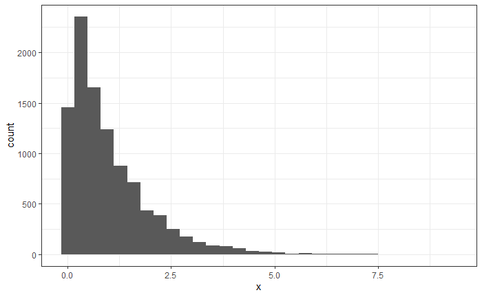
3.3
Now overlay the density of a $ \text{Expo}(1) $ to your histogram. Does the observed data appear to match the theoretical distribution?
Solution: We can use the additional argument aes(y = ..density) in the call to geom_histogram to get a density plot.
To plot the line of the Exponential density, we create a data frame expodf.
expodf <- data.frame(
	x = seq(0, 10, 0.01),
	y = dexp(seq(0, 10, 0.01), 1)
)

ggplot(x, aes(x = x)) +
	geom_histogram(aes(y = ..density..)) +
	geom_line(data = expodf, aes(x = x, y = y), color = "red")
4 Linear regression
This problem explores linear regression using the stats package’s lm command and via matrix operations. We will use the iris dataset.
4.1
Create a binary variable within iris for whether the species of each flower is setosa (i.e. it should be 1 if the flower is setosa and 0 otherwise). Call this variable setosa.
Solution: This example demonstrates this operation in base R or with dplyr.
iris$issetosa <- c(iris$Species == "setosa")
# dplyr
iris_dplyr <- iris %>%
	mutate(issetosa = c(Species == "setosa"))
4.2
Use the lm command to run a regression of setosa on all variables within iris except the Species variable. Save the model by the name lm1. (Note: you can use the documentation for lm for help. View it by entering ?lm in the console).
Solution:
lm1 <- lm(issetosa ~ . - Species, iris)
4.3
Find the “regression coefficients” by running lm1$coefficients or coef(lm1).
Solution: You should get the following result.
 (Intercept) Sepal.Length  Sepal.Width Petal.Length  Petal.Width
  0.11822289   0.06602977   0.24284787  -0.22465712  -0.05747273
4.4
Replicate the above with matrix operations.
Create a data frame called X which has our “predictor variables” (everything in iris except Species and setosa).
Add a column to X of all 1s (this should be to the left of all other columns). (Note: if you’re stuck on how to do this with data.frame(), also try cbind())
Make X into a matrix (hint: as.matrix()). Then, make a vector (which is just a 1D matrix) called y which has the response variable, setosa.
The following matrix operations should return the same coefficients as we found in 4.3. Check that this is the case
\[ \left(\mathbf{X}^T\mathbf{X} \right)^{-1}\mathbf{X}^T\mathbf{y}. \]
Solution:
iris_mat <- cbind(1, iris)
iris_mat <- iris_mat[1:5] %>% as.matrix()
x <- iris_mat

solve(t(x) %*% x) %*% t(x) %*% as.matrix(iris$issetosa)
You should get the following result:
                    [,1]
1             0.11822289
Sepal.Length  0.06602977
Sepal.Width   0.24284787
Petal.Length -0.22465712
Petal.Width  -0.05747273
Miscellaneous Advice
Everything you want to know about R Markdown can be found in this documentation: R Markdown Cookbook
A cheat sheet is also provided here: R Markdown Cheat Sheet
I’ve included some of the more important notes for STAT 111 here.
Setup for LaTeX
The easiest way to go about this is useing the tinytex package to install TinyTeX. You can do this with
# install.packages("tinytex")
tinytex::install_tinytex()
Replicating “random” variables
In order to set the RNG to be replicable, use set.seed(), where the argument is some number of your choosing.
Chunk options
When creating R chunks, you can alter the settings by adding additional fields to the header of the chunk. Here are some useful settings:
echo: Set toF(equivalent toFALSE) to have the results of code chunks display in the output file while the code chunk is hidden.include: Set toFto hide a code chunk. The chunk will still evaluate, but will be hidden in the file. This is different fromecho = Fbecauseinclude = Fwill not include graphs.eval: Set toFto have code be rendered in the output but not evaluated.message: Set toFto suppress messages from displaying. Works well withinclude = Fwhen loading libraries.warning: Set toFto suppress warnings from displaying.cache: See Time-saving measures
For example, if I wanted to run a code chunk to disaply a graph without including
all the code in the final document, I would change the content within the
brackets starting the code chunk to be {r, echo = F}. The comma after r is
important to include!
To globally alter chunk settings, use knitr::opts_chunk$set(...), where the
ellipses are replaced with the settings you want. A good example of this is found
in the default R Markdown loaded when you create a new .Rmd file in RStudio.
Time-saving measures
When knitting R Markdown files, PDF files are processed more slowly than HTML
files. When drafting homework, it’s useful to check your LaTeX (e.g., making
sure there aren’t any formatting errors) using HTML as the output before
finalizing the file as a PDF. You can do this by modifying the output field in
the header of the R Markdown file. By changing the header to read output:
html_document (or selecting HTML when creating the file), the file will knit as
an HTML. To switch to a PDF, use output: pdf_document.
Additionally, some psets will require running simulations with many repetitions. To prevent the code from running these simulations every time you knit, you can adjust the header for R code chunks to cache the results of the chunk. This will prevent the chunk from executing in subsequent knits if it is detected that the contents of the file have not been modified.
# E.g., {r cache_example, cache = T}
However, it is also possible to manually save files. This is useful because using
caching can come with caveats and you may invalidate your cache unexpectedly. To
manually save R objects, use saveRDS and readRDS.
# Let `helium` be the R object of interest
# You can name the file anything you want
saveRDS(helium, file = "helium.RDS")
helium <- readRDS(file = "helium.RDS")
Help
For functions, you can get view documentation by using a question mark. For
example, ?replicate.
You can also view the contents of a function by entering only the function name, no parentheses. This is useful for troubleshooting custom functions.